What is the real, physical, display resolution of my VR headset?
I have written a long article about the optical properties of (then-)current head-mounted displays, one about projection and distortion in wide-FoV HMDs, and another one about measuring the effective resolution of head-mounted displays, but in neither one of those have I looked into the actual display resolution, in terms of hard pixels, of those headsets. So it’s about time.
The short answer is, of course, that it depends on your model of headset. But if you happen to have an HTC Vive, then have a look at the graphs in Figures 1 and 2 (the other headsets behave in the same way, but the actual numbers differ). Those figures show display resolution, in pixels/°, along two lines (horizontal and vertical, respectively) going through the center of the right lens of my own Vive. The red, green, and blue curves show resolution for the red, green, and blue primary colors, respectively, determined this time not by my own measurements, but by analyzing the display calibration data that is measured for each individual headset at the factory and then stored in its firmware.
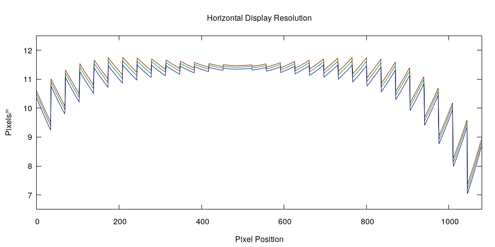
Figure 1: Resolution in pixels/° along a horizontal line through my Vive’s right lens center, for each of its 1080 horizontal pixels, for the three primary colors (red, green, and blue).
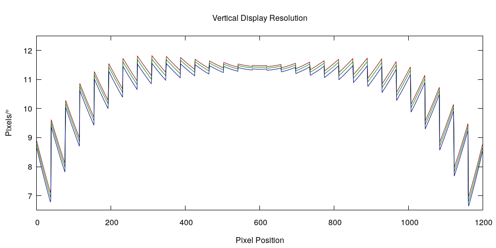
Figure 2: Resolution in pixels/° along a vertical line through my Vive’s right lens center, for each of its 1200 vertical pixels, for the three primary colors (red, green, and blue).
At this point you might be wondering why those graphs look so strange, but for that you’ll have to read the long answer. Before going into that, I want to throw out a single number: at the exact center of my Vive’s right lens (at pixel 492, 602), the resolution for the green color channel is 11.42 pixels/°, in both the horizontal and vertical directions. If you wanted to quote a single resolution number for a headset, that’s the one I would go with, because it’s what you get when you look at something directly ahead and far away. However, as Figures 1 and 2 clearly show, no single number can tell the whole story.
And now for the long answer. Buckle in, Trigonometry and Calculus ahead.
So, why do the resolution graphs look so exquisitely weird? The fact that resolution varies across the display is not that surprising, and that the resolutions for the three primary colors are different isn’t either, once you think about it, but what about those sawteeth? In order to understand what’s going on here, we have to have a close look at how modern VR headsets render 3D environments into pairs of 2D pictures, and then map those pictures onto their left and right displays.
One of the main innovations that made today’s commercial headsets possible was the idea to ditch complex, heavy, and expensive optics, and correct for the imperfections of simple, light, and cheap single lenses, namely geometric distortion and chromatic aberration, in software. These corrections are done by appending an additional processing step to the end of the standard 3D rendering pipeline. Instead of rendering 3D environments directly to the display, modern VR headsets first render 3D environments into intermediate images, using standard (skewed) perspective projection, and then warp those intermediate images onto the actual displays using non-linear correction functions that cancel out the distortions caused by the lenses that are necessary to view near-eye screens.
Step 1: Rendering to Intermediate, Rectilinear Image
In detail, the first rendering step works like this. Each VR headset has stored in its firmware the per-eye projection parameters (horizontal and vertical field of view, or FoV) needed to render appropriate views of 3D environments, and a recommended pixel size for the intermediate image (1512×1680 for the Vive). For my Vive’s right eye, the FoV parameters are as follows: left=-1.24627, right=1.39228, bottom=-1.46862, and top=1.46388. These values are in so-called tangent space, to be compatible with 3D graphics libraries. Converted to angles, they look like this: left=51.257°, right=54.312°, bottom=55.749°, and top=55.662°. Why are they not symmetric? Left and right values are different to “skew” each eye’s FoV to the outside, to provide more peripheral vision at the cost of stereo overlap. Top and bottom values are different due to manufacturing tolerances. All of these values were measured, individually for each headset, at the factory.
At this point you might be tempted to simply add up the two halves of the horizontal and vertical FoVs and claim a total of 105.569°x111.411°, but that would be rash. This rectangle is an upper limit on the headset’s real FoV, but not necessarily the actual size, as not all pixels of the intermediate image may end up on the real display, and not all of those pixels might be visible to the user.
Let’s imagine for a moment that there are no lenses, and that the intermediate image is displayed directly. What would be its resolution in pixels/°? It might seem tempting to divide total number of pixels by total FoV, yielding 14.322 pixels/° horizontally and 15.079 pixels/° vertically. But that would be wrong. The problem is that resolution is not uniform across the image, due to the image being conceptually flat. Consider Figure 3: two identical-size pixels, one directly ahead of the eye and one off to the side, cover two different angles α1 and α2.
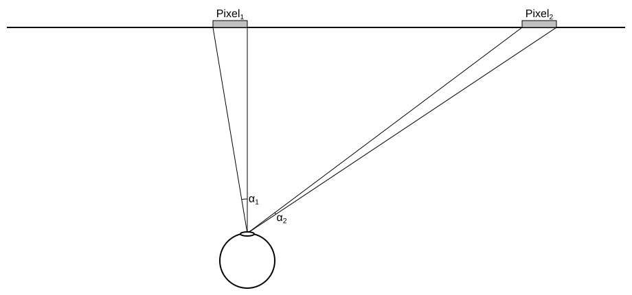
Figure 3: Resolution in pixels/° varies across flat displays, as identical-size pixels cover different angles depending on their position.
In general, if one axis of an image is N pixels long and covers a tangent-space FoV from x0 to x1, then the range of angles covered by pixel n (with n between 0 and N-1) is α1-α0 where α0=tan-1(n⋅(x1-x0)/N+x0) and α1=tan-1((n+1)⋅(x1-x0)/N+x0), yielding a resolution of 1/(α1-α0). Hold it, this is much easier to plot using differentials.
From the preceding paragraph, the function relating pixel index to angle is α(n)=tan-1((n+0.5)⋅(x1-x0)/N+x0), with 0.5 added to n to calculate pixel center angle. The derivative of tan-1(x) is, conveniently, 1/(1+x2), for a total derivative of d/dn α(n)=((x1-x0)/N)/(1+((n+0.5)⋅(x1-x0)/N+x0)2). Inverting this and converting from radians to degrees gives a resolution at pixel position n of (π/180)/(d/dn α(n)) pixels/°. Plugging in the values received from my Vive and plotting the function results in Figure 4 (as there is no lens and therefore no chromatic aberration, the resolution curves for the three primary colors collapse into one):

Figure 4: Horizontal resolution of right-eye intermediate image in pixels/°, based on parameters received from my own Vive.
This picture tells a lot. For one, that flat intermediate images are a poor fit for VR rendering, as resolution increases by a factor of 2.5 to 3 between the center and the edges, meaning that a disproportionally large amount of the rendered pixels are allocated to the periphery, where they are not particularly useful. While projection onto flat planes is inherent in 3D graphics, nobody said that the planes had to be flat in 3D affine space. Using flat planes in 3D projective space yields a nice rendering trick, but that’s a topic for another article.
Anyway, does the curve in Figure 4 remind anyone of anything? Imagine scaling Figure 4 vertically by a factor of 3.5, then taking scissors to it, and cutting it into 31 identical-sized vertical strips, and then shifting those strips downwards by increasing amounts going from the center outwards. Now compare that mental image to Figure 1. See a resemblance? Spoiler alert: that’s exactly what’s going to happen in the next rendering step.
Step 2: Non-linear Correction for Lens Distortion and Chromatic Aberration
The secret to successful lens distortion correction lies in measuring that distortion during a calibration step. This is done, ideally for each headset individually, at the factory. The exact calibration setup may vary, but one option is using a calibrated camera, like the one I used in the experiments described in this article, to capture how known calibration images shown on a headset’s displays would appear to a viewer.
The gist of it is this: to create a convincing illusion of virtual reality, if a virtual object is located in a certain direction from the virtual viewer, then that virtual object needs to be presented to the real viewer along the exact same direction. In other words: for each pixel on a headset’s display, we need to know the exact direction at which that pixel appears to the viewer wearing the headset. And the easiest way to express that direction is by horizontal and vertical tangent space coordinates.
Now, if calibration gives us a map of tangent space directions for every display pixel, how do we assign a color to any one of those pixels during rendering? Fortunately, we already have an image that represents the virtual 3D environment in tangent space: the intermediate image that was generated in step 1. This yields a simple procedure for lens distortion correction: for each display pixel, look up its tangent space coordinates in the calibration map, and then copy the pixel that has the same tangent-space coordinates in the intermediate image. Due to the intermediate image’s rectilinear structure, that last part is a very simple look-up.
And even better: the same procedure can also correct for chromatic aberration. Instead of storing a single tangent space coordinate for each display pixel, we store three: one each for the red, green, and blue color components. Because the three colors get diffracted to different degrees by the same lens, their tangent space coordinates for the same pixel will be different.
This is all really nice, but a remaining problem is how to represent the calibration map. In principle, the map is an image with 1080×1200 pixels (in the Vive’s case), and six components per pixel: one tangent space (x, y) for each of the three colors. For technical reasons, representing the map like this is not very efficient in terms of rendering performance. A better approach, and the one used by the Vive and all other OpenVR headsets, is to simplify the map to a so-called distortion mesh of NxM identical-sized (in display space) rectangles, storing per-color tangent space coordinates only at the corners of those rectangles, and interpolating between the corner values across each rectangle. This is better because it is compact (N and M can be small) and performs well because modern graphics cards are really good at drawing, and interpolating values across, rectangles. For illustration, Figure 5 shows my Vive’s right-screen green channel distortion mesh, both in display space and tangent space, and, in the latter case, superimposed over the rectangular boundaries of the intermediate image.
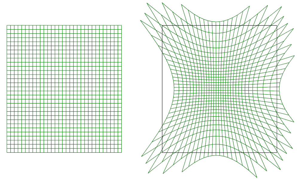
Figure 5: My Vive’s right-screen green-channel distortion mesh. Left: Mesh in display space, showing 31×31 identical rectangles. Right: Mesh in tangent space superimposed over intermediate image’s FoV (black rectangle). Only parts of the mesh contributing to the displayed image are drawn.
Figure 5 shows several interesting things. Most importantly, it shows that the Vive’s lens causes quite a bit of pincushion distortion. The mesh cells close to the lens’s center are compressed, whereas those around the periphery are stretched. This has the intended effect of allocating more real display pixels to the important central focus area, and fewer to the periphery, than in the intermediate image. The lens, in other words, more than cancels out the unfortunate resolution distribution seen in Figure 4, evidenced by the fact that the final display resolution is higher in the center than in the periphery, as seen in Figures 1 and 2.
Resolution is evened out by the stretching of the mesh cells in tangent space. A small cell will allocate a small number of intermediate-image pixels to a fixed-size area of the real display, increasing local resolution, whereas a stretched cell will stuff a larger number of pixels into the same fixed-size area, decreasing local resolution. This explains the inverted resolution distribution in Figures 1 and 2, but not yet the presence of sawteeth.
Those, as it turns out, have a simple explanation: graphics cards interpolate values from the corners of rectangles across their interiors using linear interpolation, meaning that the resulting distortion map is a piecewise linear function. And the derivative of a piecewise linear function is a piecewise constant function with discontinuous jumps between the pieces. Those constant pieces, modulated by the gradually varying local resolution inside each grid cell, exactly cause the appearance of the graphs in Figures 1 and 2. The discontinuities in derivative are not a problem, as viewers don’t see the derivatives, only the functions themselves. And those are continuous everywhere.
Another interesting observation from Figure 5 is that the overlap between the distortion mesh in tangent space and the intermediate image is not perfect. Parts of the intermediate image are not covered (the lens-shaped area along the left border), and parts of the distortion mesh fall outside the intermediate image. The first part means that a part of the intermediate image, and by extension its FoV, is not seen by the viewer; the second part means that parts of the real display do not receive valid image data and are therefore unusable.
The Vive’s designers made an interesting decision here: they extended the left boundary of the right intermediate image beyond the left edge of the real right display (and vice versa for the left display), in order to gain some precious stereo overlap with the other eye. FoV is not extended when looking directly to the left, as there are no more display pixels there, but is extended when looking to the left and slightly up or down. The “downside” is the odd-looking “partial eclipse” shape of the Vive’s rendered intermediate image with two missing chunks on the inner edges.
One last thing to mention: where does the recommended intermediate image size of 1512×1680 pixels come from? It was chosen so that the resolution of the intermediate image, after feeding it through the distortion mesh, approximately matches the resolution of the real screen in the lens center area, to minimize aliasing from the resampling procedure that’s inherent in warping one raster image onto another raster image. Specifically, the intermediate image’s resolution at the exact lens center is slightly lower than the real display’s (10.01 pixels/° vs. 11.42 pixels/°), but the intermediate image quickly overtakes the real display going outwards, see Figure 6.
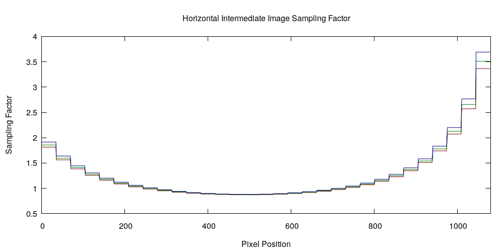
Figure 6: Distribution of sampling factors, i.e., number of intermediate-image pixels collapsed into one real display pixel, along a horizontal line through the center of my Vive’s right lens. The sampling factor stays close to 1.0 in a relatively large area around the lens’s center, dipping to 0.876 at the exact center, and then grows quickly.
In conclusion: quantifying the real, physical, resolution of VR headsets (what I did here for the Vive applies in the same way to all the others) is a complex issue, as it depends on the optical properties of the lens, the representation and resolution of the calibration map (mesh vs. image vs. analytic function), and of course on the pixel count of the real display and its real field of view. But, as it turns out, there is a reasonable way to boil it down to a single number for rough comparisons, by quoting the green-channel resolution at the exact center of the lens.

Very nice write-up, I did notice the matching curves before you mentioned it, kind of like a crime drama where there are no coincidences 😉 Manufacturers still talk about actual panel PPI and resolution, which have been kind of pointless since the very beginning as it’s not what the end user actually sees.
I remember with the DK1 that I swapped lenses and drew the images circles I could see to calculate the abysmal amount of pixels we actually saw. It was a hopeless battle to convince other Reddit users that we should not do a straight comparison to other headsets from the panel alone, but eh, I gave up on that as Eternal September settled in.
Good job extracting the firmware calibration data 🙂 Must have been nice to work with confirmed and ~exact values 😀
Well, the values are only “confirmed and exact” if you believe that the firmware isn’t lying. 🙂 But in this case I believe it, as the values match what I’ve measured myself. The firmware values have higher resolution.
It wasn’t hard extracting them. They are part of the parameters required to render correctly to the HMD, and OpenVR’s driver interface is not coy about them at all. 😉 I’ve been using them for Vrui rendering for years, but never bothered doing this math.
Thank you for the write-up. I always enjoy your posts.
On Figures 1 & 2, the angular resolution for the red/green/blue primary colors match closely. Due to the Pen-tile display on the Vive with half the red/blue pixel coverage, wouldn’t the red/blue channels to only provide ~50% the angular resolution relative to the green channel? Roughly 5.5 red/blue ppd at the center
I didn’t take subpixel layout into account for this write-up. This analysis was driven by the calibration data handed to VR applications by the HMD’s firmware, and subpixel layout, or at least subpixel density, is not part of those data.
It would be 1/sqrt(2) which is about 71% of the linear resolution, or 8.08 PPD. The grid for red and blue is rotated by 45 degrees.
Very interesting read. Altough even as a engineer I am too dumb to understand all.
You say there is a “reasonable way to boil it down to a single number for rough comparisons”, but doesnt compare, only showing vive number.
I want number for all HMD to use on forums as a know it all, lol. Would be nice, but I know the amount of work this would take.
Thanks.
If you happen to have a Rift, you could extract OpenVR-format calibration data from it and send it, as I detail in this comment over on reddit. That would allow me to do the same analysis for Rift.
Pingback: The Display Resolution of Head-mounted Displays – VRomit's World
Pingback: The Display Resolution of Head-mounted Displays, Revisited | Doc-Ok.org
Pingback: Visual Simulation of the Resolution of VR Headsets | Doc-Ok.org