One of the mysteries of the modern age is the existence of two distinct lines of graphics cards by the two big manufacturers, Nvidia and ATI/AMD. There are gamer-level cards, and professional-level cards. What are their differences? Obviously, gamer-level cards are cheap, because the companies face stiff competition from each other, and want to sell as many of them as possible to make a profit. So, why are professional-level cards so much more expensive? For comparison, an “entry-level” $700 Quadro 4000 is significantly slower than a $530 high-end GeForce GTX 680, at least according to my measurements using several Vrui applications, and the closest performance-equivalent to a GeForce GTX 680 I could find was a Quadro 6000 for a whopping $3660. Granted, the Quadro 6000 has 6GB of video RAM to the GeForce’s 2GB, but that doesn’t explain the difference.
Intrinsic camera calibration, as I explained in a previous post, calculates the projection parameters of a single Kinect camera. This is sufficient to reconstruct color-mapped 3D geometry in a precise physical coordinate system from a single Kinect device. Specifically, after intrinsic calibration, the Kinect reconstructs geometry in camera-fixed Cartesian space. This means that, looking along the Kinect’s viewing direction, the X axis points to the right, the Y axis points up, and the negative Z axis points along the viewing direction (see Figure 1). The measurement unit for this coordinate system is centimeters.
Figure 1: Kinect’s camera-relative coordinate system after intrinsic calibration. Looking along the viewing direction, the X axis points to the right, the Y axis points up, and the Z axis points against the viewing direction. The unit of measurement is centimeters.
ShowEarthModel is one of the example programs shipped with the Vrui VR development toolkit. It draws a simple texture-mapped virtual globe, and can be used to visualize global geophysical data sets — specifically those containing subsurface data, as the globe can be drawn transparently. However, ShowEarthModel is not packaged with any data sets, primarily to keep the download size small, but also for licensing reasons. Out of the box, it only contains a fairly low-resolution color-mapped Earth topography texture (which can be changed, but that’s a topic for another post).
Since it’s one of the most common requests, here are the steps to download up-to-date earthquake data from the ANSS online catalog:
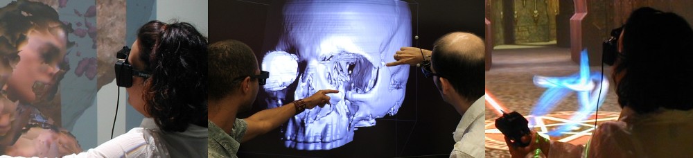
Qin-zhu, and a small army of other researchers, just published a Science paper about their work on the meteorite. Qin-zhu then asked me to create a few short movies showing 3D visualizations of several of those scans, from both flavors of CT, to go along with the release of the Science paper on 12/20/2012. I used our 3D Visualizer software, which is originally aimed at immersive environments such as CAVEs, but works well on desktop workstations as well, to load the 3D data sets, and visualize them using direct volume rendering.
We are currently involved in an NSF-funded project to study the changes in global ocean flow patterns in response to past climate change, specifically the difference in flow patterns between the last glacial maximum (otherwise known as the “Ice Age”, ~25000 years ago) and the Holocene (otherwise known as “today”).
In layman’s terms, the basic idea is to use differences in the chemical composition, particularly the abundance of isotopes of carbon (13C) and oxygen (18O), of benthiccore samples collected from the ocean floor all around the world to establish correlations between sampling sites, and from that derive a global flow model that best explains these correlations. (By the way, 13C is not the carbon isotope used in radiocarbon dating; that honor goes to 14C).
This is a multi-institution collaborative project. The core sample isotope ratios are collected and collated by Lorraine Lisiecki and her graduate students at UC Santa Barbara, and the mathematical method to reconstruct flow patterns based on those samples is developed by Jake Gebbie at Woods Hole Oceanographic Institution. Howard Spero at UC Davis is the overall principal investigator of the project, and UC Davis’ contribution is visualization and analysis software, building on the strengths of the KeckCAVES project. I’ve posted previously about our efforts to construct low-cost immersive display systems at our collaborators’ sites so that they can use the visualization software developed by us in its native habitat, and also collaborate with us and each other remotely in real-time using Vrui’s collaboration infrastructure.
So here is the first major piece of visualization software developed specifically for this project. It was developed by Rolf Westerteiger, a visiting PhD student from Germany, based on the Vrui VR toolkit. Here is Rolf himself, using his application in the CAVE:
PhD student Rolf Westerteiger using his immersive visualization application in the KeckCAVES CAVE.
This application reads a database of core sample compositions created by Lorraine Lisiecki, and a reconstructed 3D flow field created by Jake Gebbie, and puts both into a global three-dimensional context. The software shows a block model of the Earth’s global ocean floor (at the same resolution as the 3D flow field, and vertically exaggerated by a significant factor), and allows a user to interactively query and explore the 3D flow.
The primary flow visualization method is line integral convolution (LIC), which creates dense and intuitive visualizations of complex flows. As LIC works best when applied to 2D surfaces instead of 3D volumes, Rolf’s application is based on a set of interactively controllable surfaces (one sphere of constant depth, two cones of constant latitude, two semicircles of constant longitude) which slice through the implicitly-defined 3D LIC volume. To indicate flow direction, the LIC texture is animated by cycling through a phase offset, and color-coded by either flow velocity or water temperature.
The special thing about this LIC visualization is that the LIC textures are not pre-computed, but generated in real time using the GPU and a set of GLSL shaders. This allows for even more interactive exploration than shown in this first result; a user could specify arbitrary slicing surfaces using tracked 3D input devices, and see the LIC pattern displayed on those surfaces immediately. From our experience with the 3D Visualizer software, which is based on very similar principles, we believe that this will lead to a very powerful exploratory tool.
A secondary flow visualization method are tracer particles, which can be injected into the global ocean at arbitrary positions using a tracked 3D input device, and leave behind a trail of their past positions. Together, these two methods provide rich insight into the structure of these reconstructed flows, and especially their evolution over geologic time.
A third visualization method is used to put the raw data that were used to create the flow models into context. A set of labels, one for each core sample in the database, and each showing the relative abundance of the important isotope ratios, are mapped onto the virtual globe at their proper positions to enable visual inspection of the flow reconstruction method.
Unfortunately, Rolf had to return to Germany before we were able to film a video showing off all features of his visualization application, so I had to make a video with myself standing in for him:
The next development steps are to replace the ocean floor block model read from the flow file with a high-resolution bathymetry model (see below), and to integrate the visualization application with Vrui’s remote collaboration infrastructure such that it can be used by all collaborators for virtual joint data exploration sessions.
Global high-resolution bathymetry model at 75x vertical exaggeration. View is centered on Northern Atlantic.
I’ve already mentioned KeckCAVES‘ involvement in NASA‘s newest Mars mission, the Mars Science Laboratory, in a previous post, but now I have an update. Dawn Sumner, UC Davis‘ member of the Curiosity science team, was interviewed last week for “Onward California,” which I guess is some new system-wide outreach and public relations effort to get the public’s mind off last fall’s “unpleasantries.” Just kidding UC, you know I love you.
Anyway… Dawn decided that the best way to talk about her work on Mars would be to do the interview in the CAVE, showing how our software, particularly Crusta Mars, was used during the planning stages of the mission, specifically landing site selection. I then suggested that it would be really nice to do part of the interview about the rover itself, using a life-size and high-resolution 3D model of the rover. So Dawn went to her contacts at the Jet Propulsion Laboratory, and managed to get us a very detailed 3D model, made of several million polygons and high-resolution textures, to load into the CAVE.
What someone posing with a life-size 3D model of the Mars Curiosity rover might look like.
As it so happens, I have a 3D mesh viewer that was able to load and render the model (which came in Alias|Wavefront OBJ format), with some missing features, specifically no specularity and bump mapping. The renderer is fast enough to draw the full, undecimated mesh at sufficient frame rate for immersive display, around 30 frames per second.
The next problem, then, was how to film the beautiful rover model in the CAVE without making it look like garbage, another topic about which I’ve posted before. The film team, from the Department of the 4th Dimension, fortunately was on board, and filmed the interview in several segments, using hand-held and static camera setups.
We have pretty much figured out how to film hand-held video using a secondary head tracker attached to the camera, but static setups where the camera is outside the CAVE, and hence outside the tracking system’s range, always take a lot of trial and error to set up. For good video quality, one has to precisely measure the 3D position of the camera lens relative to the CAVE and then configure that in the CAVE software.
Previously, I used to do that by guesstimating the camera position, entering the values into the configuration file, and then using a Vrui calibration utility to visually judge the setup’s correctness. This involves looking at the image and why it’s wrong, mentally changing the camera position to correct for the wrongness, editing the configuration file, and repeating the whole process until it looks OK. Quite annoying that, especially if there’s an entire film crew sitting in the room checking their watches and rolling their eyes.
After that filming session, I figured that Vrui could use a more interactive way of setting up CAVE filming, a user interface to set up and configure several different filming modes without having to leave a running application. So I added a “filming support” vislet, and to properly test it, filmed myself posing and playing with the Curiosity rover (MSL Design Courtesy NASA/JPL-Caltech):
Pay particular attention to the edges and corners of the CAVE, and how the image of the 3D model and the image backdrop seamlessly span the three visible CAVE screens (left, back, floor). That’s what a properly set up CAVE video is supposed to look like. Also note that I set up the right CAVE wall to be rendered for my own point of view, in stereo, so that I could properly interact with the 3D model and knew what I was pointing at. Without such a split-CAVE setup, it’s very hard to use the CAVE when in filming mode.
The filming support vislet supports head-tracked recording, static recording, split-CAVE recording (where some screens are rendered for the user, and some for the camera), setting up custom light sources, and a draggable calibration grid and input device markers to simplify calibrating a static camera setup when the camera is outside the tracking system’s range and cannot be measured directly.
All in all, it works quite well, and is a significant improvement over the previous setup method. It is now possible to change filming modes and camera setups from within a running application, without having to exit, edit configuration files, and restart.
I started working on low-cost VR, that is, cheap (at least compared to a CAVE or other high-end system) professional-grade holographic display systems about 4 1/2 years ago, after seeing one at the 2008 IEEE VR conference. It consisted of a first generation DLP-based projection 3D TV and a NaturalPointOptiTrack optical tracking system. I put together my own in Summer 2008, and have been building, or helped others building, more at a steadily increasing rate — one in my lab, one in our med school, one at UC Berkeley, one at UC Merced, one at UC Santa Barbara, a handful more at NASA labs all over the country, and probably some I don’t even know about. Here’s a video showing me using one to explore a CAT scan of a patient with a nasty head fracture:
Back then, I created a new subsite of my web site dedicated to low-cost VR, with a detailed shopping list and detailed installation and configuration instructions. However, I did not update either one for a long time after, leading to a very outdated shopping list and installation instructions that were increasingly divergent from state-of-the-art approaches.
But that has changed recently. As part of an NSF-funded project on paleoceanography, we promised to install two such systems at our partner institutions, University of California, Santa Barbara, and Woods Hole Oceanographic Institution. I installed the first one a couple of months ago. Then, I currently have two exchange students from the University of Georgia (this Georgia, not that Georgia) who came here to learn how to build these systems in order to build one for their department at home. To train them, I rebuilt my own system from scratch, let them take the lead on rebuilding the one at our medical school, and right now they’re on the east coast to install the new system at WHOI.
Observing “newbies” following my guide trying to build a system from scratch allowed me to significantly improve the instructions, to the point that I believe they’re now comprehensive and can be followed by first-time builders with some computing knowledge. I also updated the shopping list to again represent a currently-available system, with current prices.
So the bottom line is that I now feel comfortable to let people go wild with the low-cost VR subsite and build their own display systems. If no existing equipment (computers, 3D TVs, …) can be used, a very nice, large (65″ TV), and powerful system can be built for around $7000, depending on daily deals. While not exactly cheap-cheap, one has to keep in mind that this is a professional-grade system, fit for scientific and other serious uses.
I should mention that we have an even lower-cost design, replacing the $3500 optical tracking system with a $150 Razer Hydra controller, but there’s a noticeable difference in functionality between the two. I should also mention that there’s a competing design, the IQ Station, but I believe that ours is better (and I’m not biased at all!).
While I was in Santa Barbara recently to install a low-cost VR system, I also took the chance to visit the Allosphere. One of the folks behind the Allosphere is Tobias Höllerer, a computer science professor at UCSB who I’ve known for a number of years; on this visit, I also met JoAnn Kuchera-Morin, the director of the Allosphere Research Facility, and Matthew Wright, the media systems engineer.
Allosphere Hardware
The Allosphere is an audacious design for a VR environment: a sphere ten meters in diameter, completely illuminated by more than a dozen projectors. Visitors stand on a bridge crossing the sphere at the equator, five meters above ground. While I did take my camera, I forgot to take good pictures; Figure 1 is a pretty good impression of what the whole affair looks like.
Figure 1: What the Allosphere kinda looks like. Image taken from the Marvel Movies Wiki.
Earlier this year, I branched out into augmented reality (AR) to build an AR Sandbox:
Photo of AR Sandbox, with a central “volcano” and several surrounding lakes. The topographic color map and contour lines are updated in real time as the real sand surface is manipulated, and virtual water flows over the real sand surface realistically.
I am involved in an NSF-funded project on informal science education for lake ecosystems, and while my primary part in that project is creating visualization software to drive 3D displays for larger audiences, creating a hands-on exhibit combining a real sandbox with a 3D camera, a digital projector, and a powerful computer seemed like a good idea at the time. I didn’t invent this from whole cloth; the project got started when I saw a video of such a system done by a group of Czech students on YouTube. I only improved on that design by adding better filters, topographic contour lines, and a physically correct water flow simulation.
The idea is to have these AR sandboxes as more or less unsupervised hands-on exhibits in science museums, and allow visitors to informally learn about geographical, geological, and hydrological principles by playing with sand. The above-mentioned NSF project has three participating sites: the UC Davis Tahoe Environmental Research Center, the Lawrence Hall of Science, and the ECHO Lake Aquarium and Science Center. The plan is to take the current prototype sandbox, turn it into a more robust, museum-worthy exhibit (with help from the exhibit designers at the San Francisco Exploratorium), and install one sandbox each at the three sites.
But since I published the video shown above on YouTube, where it went viral and gathered around 1.5 million views, there has been a lot of interest from other museums, colleges, high schools, and private enthusiasts to build their own versions of the AR sandbox using our software. Fortunately, the software itself is freely available and runs under Linux and Mac OS X, and all the hardware components are available off-the-shelf. One only needs a Kinect 3D camera, a data projector, a recent-model PC with a good graphics card (Nvidia GeForce 480 et al. to run the water simulation, or pretty much anything with water turned off) — and an actual sandbox, of course.
In order to assist do-it-yourself efforts, I’ve recently created a series of videos illustrating the core steps necessary to add the AR component to an already existing sandbox. There are three main steps: two to calibrate the Kinect 3D camera with respect to the sandbox, and one to calibrate the data projector with respect to the Kinect 3D camera (and, by extension, the sandbox). These videos elaborate on steps described in words in the AR Sandbox software’s README file, but sometimes videos are worth more than words. In order, these calibration steps are:
Step 1 is optional and will get a video as time permits, and steps 3, 6, and 8 are better explained in words.
Important update: when running the SARndbox application, don’t forget to add the -fpv (“fix projector view”) command line argument. Without it, the SARndbox won’t use the projector calibration matrix that you so carefully calibrated in step 7. It’s in the README file, but apparently nobody ever reads that. 😉
The only component that’s completely left up to each implementer is the sandbox itself. Since it’s literally just a box of sand with a camera and projector hanging above, and since its exact layout depends a lot on its intended environment, I am not providing any diagrams or blueprints at this point, except a few photos of our prototype system.
Basically, if you already own a fairly recent PC, a Kinect, and a data projector, knock yourself out! It should be possible to jury-rig a working system in a matter of hours (add 30 minutes if you need to install Linux first). It’s fun for the whole family!